| June Stenzel |
| PHYS-425-501 Senior Lab |
| Department of Physics and Astronomy, Texas A&M University, College Station, |
| Texas 77843-4242, USA |
| May 1, 2018 |
Muons radiation occurs as a result of cosmic rays striking our upper atmosphere. This radiation is largely isotropic throughout the sky and is constantly incident on the Earth’s surface. In this report, we present the theory and design of an experiment which can measure these muons. Using a pair of Geiger-Müller detector tubes, we characterize the surface muon flux as a function of inclination angle, and discuss methods of analysis to draw conclusions from this data.
Cosmic rays are high-energy particles from beyond our solar system that are constantly incident on our atmosphere. They are distinct from space-sourced electromagnetic radiation, in that they are relativistic massive particles, usually individual protons or low-mass atoms. These particles are commonly observed to be in energy ranges between \(10^3\) to \(10^8\) MeV, but have been measured as high as \(3 \times 10^{20}\) MeV \(^{[1]}\). There is indication that they are a product of multiple different kinds of events, including distant supernova, or in more extreme cases, part of the output of black holes or active galactic nuclei.
When cosmic rays strike the Earth’s upper atmosphere, they trigger a shower of secondary particles to rain down to the surface. These cosmic ray secondaries consist of a number of particles, including photons, electrons, muons, nucleons, mesons, and some antimatter particles. The collision products which are actually detected on the ground are predominantly muons \(^{[2]}\).
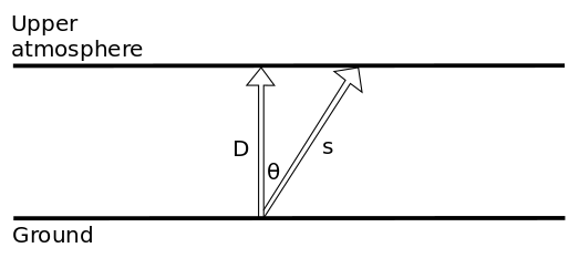
Because atmospheric muons have a mean lifetime of around 2.2 \(\mu\)s \(^{[3]}\), and they are subject to atmospheric absorption, their direct observation is affected by two key conditions. One is that measured muon intensity increases with altitude, which is one of the factors that led to Victor Hess’ Nobel prize-winning discovery of cosmic rays using electrometers mounted in balloons \(^{[4]}\). The other is that muon intensity will depend on the angle of measurement relative to the normal of the Earth’s surface, as a greater inclination angle corresponds to a greater atmospheric distance. This notion is illustrated in Figure 1.
If we consider that muons are being radiated onto the Earth uniformly from above, then the intensity of atmospheric muons will be a constant, and the muon count flux for a given angle will have a dependence on the atmospheric distance:
\[\Phi ~\sim~ \frac{1}{s^2} = \frac{\cos^2 \theta}{D^2},\]
where there is further dependence on the intensity \(I_{max}\).
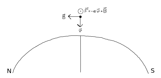
There are a number of other phenomena which slightly affect the solid-angle distribution of muon incidence. The most significant is the east-west effect, in which downward-traveling muons are pushed towards the west due to the Lorentz force of the Earth’s magnetic field,
\[\textbf{F}_{E-W} = q\textbf{v} \times \textbf{B},\]
where \(q = -e\). A depiction of this effect is shown in Figure 2.
An additional higher-order correction onto this model of muon is the latitude effect \(^{[4]}\), in which charged particles interact with the magnetic dipole field of the Earth. In this situation, the amount that a particle is deflected by the Lorentz force is proportional to both its energy, and the position of the particle relative to the Earth’s polar angle. This results in a northward shift, such that there are more muons incident near the north pole than near the south. Analytically calculating and experimentally measuring this effect is beyond the scope of this paper, and is minor enough to be neglected for our analyses.
These factors are all important to understanding how we detect muons, and also how we begin to measure cosmic rays. Muon tomography, a method of imaging using cosmic ray transmission measurements to probe the internal makeup of large objects, uses many of the same methods and principles as discussed in this paper. This practice has a wide array of applications, and in fact was recently used to detect the inner structure of the Chephren Pyramid in Giza \(^{[6]}\).
An understanding of the energies and sources of the high-energy cosmic ray events events that we measure here leads not only to better astrophysical understandings, but also to the growing field of cosmic ray astronomy, which is concerned with using charged carriers to measure otherwise undetectable astrophysical magnetic fields \(^{[5]}\).
We perform the measurements of muon incidence using a Geiger-Müller tube, which is the radiation-sensitive component in laboratory Geiger counters. The fundamental principle is that whenever charged radiation enters the interior of the tube, it triggers brief ionization of the gas inside that is read electronically as a count.
In order to measure the angular dependence of muon flux on the Earth’s surface, we use a pair of Geiger-Müller tubes. Each one is connected to the same gas flow and high-voltage power source, and they are read concurrently under the assumption that if there is a detection in each of the tubes at nearly the same time, then one muon has passed through them.
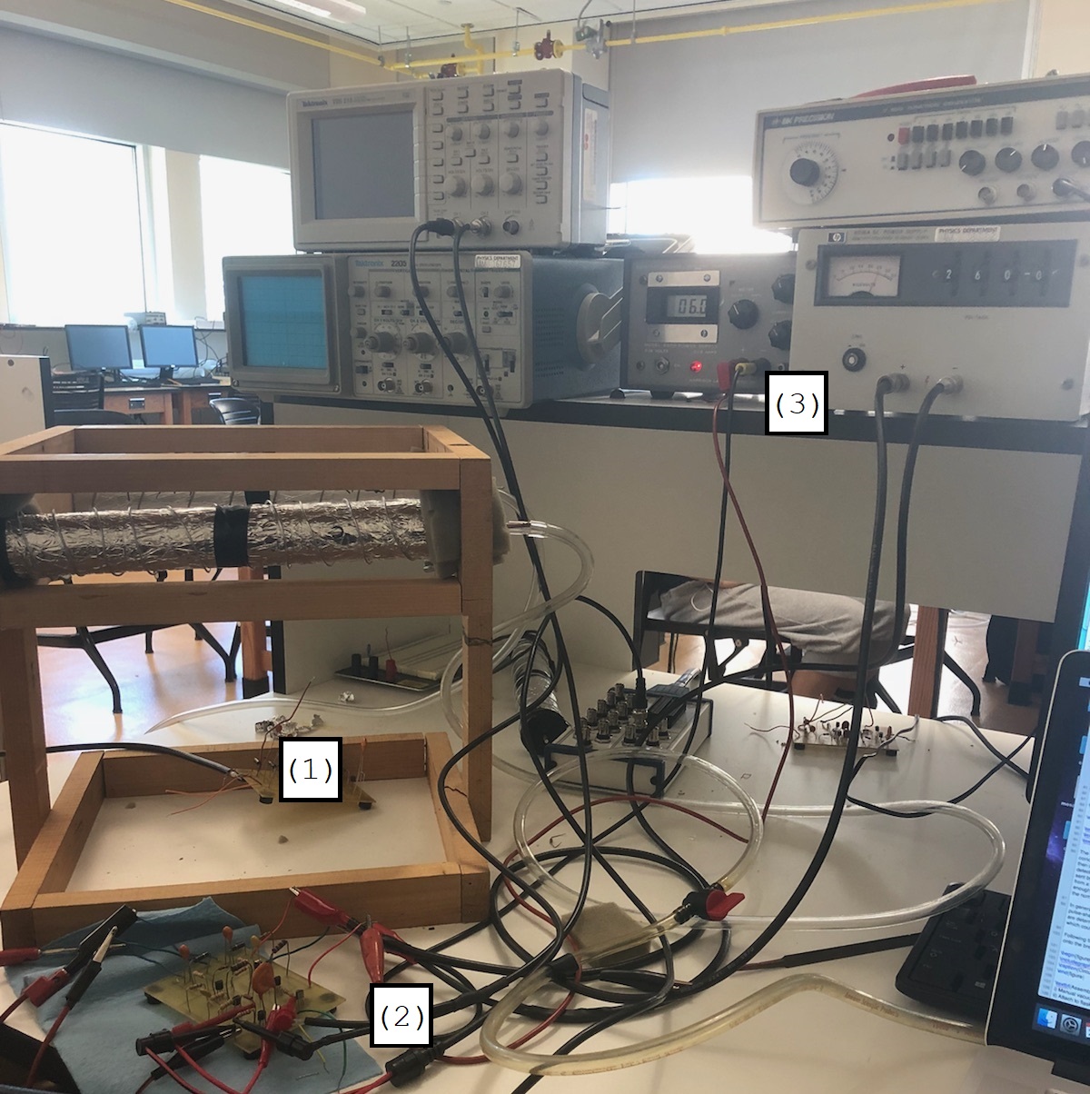
The tubes are mounted on a wooden stand, as seen in Figure 4, that can be positioned and rotated freely. This allows us to measure the muon incidence from one specific direction at a time.
Each detector tube consists of two charged concentric cylinders, and so essentially forms a large capacitor. We can calculate the capacitance of a tube, using
\[\frac{C}{L} = \frac{2 \pi k \epsilon_0}{\ln(b/a)},\]
the equation of capacitance per unit length of two concentric cylinders \(^{[8]}\), given \(a\) outer radius of wire, \(b\) inner radius of tube, and dielectric constant of helium \(k\). Then, for our tubes the capacitance is approximately \(C = 3 \times 10^{-10}\) F.
When charged radiation enters the tube, it causes the gas mixture, which we choose to be 99% helium and 1% butane, to ionize in a process called a Townsend avalanche. Such a muon event causes the tube capacitor to discharge. Electrical charge flows from the anode, a positive inner tungsten filament, to the cathode, a grounded outer shell outside the glass.
When a charged particle enters the detector, it is attracted to the anode by the large electrical potential. As it moves into the tube and ionizes the helium molecules in its path, the freed electrons are also drawn to the anode, leaving the heavier ions to continue in the gas flow. This cascade causes a significant current to momentarily flow within the tube, which is detected and logged by electronics monitoring the tubes. Because this effect is concentrated near the central wire, the region of positive ions and flowing electrons around the anode effectively increases the radius of the anode \(^{[9]}\).
It is important for the gas within the tubes to be flowing at a constant rate, so that changing flow rate does not disturb the measured detection rate. The flow must slow enough that these ionization regions are not prohibited from forming, but fast enough so that there is fresh gas to ionize whenever a new muon enters the tube. In fact, some finite "recovery period" after ionizations in the detector is inevitable due to ionized gas, and is a source of experimental error.
The 1% butane in the gas mixture serves the purpose of internal quenching. The high electric fields near the anode can cause some of the atoms to excite and emit ultraviolet light, which could cause an ionization event and thus a false count. As a heavy organic molecule, the butane serves the purpose of absorbing these ultraviolet photons and keep the helium atoms from crowding the region of the anode too closely \(^{[10]}\).
At the output of the tubes, we bubble the gas through a beaker of oil to monitor flow rate. For our measurements, we keep the flow rate in the vicinity of 1 bubble per second.
We constructed three detector tubes, with one serving as a back-up. We started by cutting cylindrical segments of glass, 12 inches in length and 2 inches in diameter. This was done by scoring the circumference of the glass tube with a diamond cutting tool, then applying pressure to break it cleanly. We then used a blowtorch to smooth the edges of the tube segment.
With a similar method, we cut 6 short segments of 7 mm diameter glass tube to a length of about 2 inches, and blowtorched the ends for smoothness. These tubes affix to both endcaps, and are the means by which gas flows through the tubes. The copper tube was placed in the center of the end cap face, and the glass tube was offset from the center by at approximately half of the radius, to make it easier to connect tubing to it.
We cut 2 inch lengths of thin copper tubing, and assembled Lucite end caps for each tube that fit snugly into either end. In each of the end caps, we made holes such for the copper and glass tubes to fit into. After wiping down the end caps, copper, and glass with methanol, we affixed the small copper and glass tubes to each of the end caps. We used a Devcon epoxy which cures at room temperature and fully solidified after 24 hours.
After those were cured, we cleaned and epoxied one of the fully-assembled end caps to one end of each of the tubes. We then threaded one end of an approximately 20 inch long strand of thin-filament tungsten wire through the copper tube. This wire was kept clean, through the use of methanol washing and rubber gloves. We crimped the end of the copper tube so as to hold the end of the wire in contact, and soldered the end of the wire to the opening of the tube. We gripped the base of the copper tube with pliers used as a heatsink to prevent the heat of the process from causing any of the the epoxy to degrade. Soldering this end piece ensured that the tungsten wire is in good electrical contact with the copper, and mades the tube airtight. We pulled on the loose wire in order to make sure that it was well-attached. We were careful to keep the wire from bending or catching on surface, as kinks in the wire would cause anomalies in the detection process.
We then threaded the free end of the tungsten wire through the other unattached glass end cap, and cleaned and epoxied that end into place as well. While this end was curing, we taped the excess length of wire to the outside of the tube, in order to prevent the wire from getting loose and fall into the tube by mistake. After curing was complete, we pulled the tungsten wire taut with an extra set of pliers, and repeated the crimping and soldering process for this end. Then, we trimmed the excess wire on each end.
![Figure 5: A schematic drawing of the fully-constructed tube (adapted from {[2]}.)](https://junestenzel.com/wp-content/uploads/tube.png)
At this stage, we connected each of three detector tubes to a vacuum pump to bring it to -30 psi relative to standard pressure. This allowed us to test for the vacuum properties of our detector and identify any leaks. For example, one of our tubes had a chip in the glass near the end cap that occurred during the glass cutting stage, which we fixed with an additional layer of epoxy.
After the tubes reached and held a negative pressure of 30 psi, we connected the two copper posts to each end of a variable autotransformer, or variac \(^{[11]}\), which is a device capable of generating high voltages. By turning up the voltage until the tungsten wire glows red for several seconds, we cleaned the wire of any trace impurities or contaminants. During setup and troubleshooting, we often tested the resistance across the two copper posts in order to ensure that the tungsten wire is undamaged and still in good contact.
Then, we wrapped the length of each of the tubes with several layers of aluminum foil. We held this foil in place with electrical tape, which we also used to cover the surface of the endcaps. This ensured that the detectors are not sensitive to light near the visible range.
We wrapped 18 AWG bus bar wire in a helix pattern around the circumference of each tube, with a length between consecutive loops of about 0.5 inches. These ends of these wires are left free on each end, and electrical tape is used to keep the coil in place and in electrical contact with the aluminum foil covering. We were careful to prevent either the bus bar wire or the aluminum foil to come in contact with the copper post, which would case an electrical short when the tube is connected to high voltage.
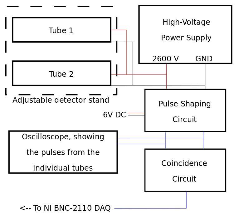
With our two tubes individually creating electrical pulses upon detection, we constructed a circuit that can both shape the high-voltage signal into a more discrete and low-power response, and perform a coincidence detection. Figure 6 shows the electrical diagram of the circuit we used. This circuit requires a 6 V power supply, independent of the high-voltage power source used to create the potential in the tubes.
![Figure 6: Schematic diagram of the signal shaping and coincidence circuits ^{[2]}.](https://junestenzel.com/wp-content/uploads/circuit.png)
The goal of the coincidence circuit is to only output a pulse when a signal is read on both input channels nearly-simultaneously. This logic amounts to simply an AND-circuit, which is implemented with transistors here, and the timescale of what is considered simultaneous for this experiment is set by the RC component at the end. With the resistance \(R = 2.2\) k\(\Omega\) and capacitance \(C = 0.01\) \(\mu\)F, the timescale here is
\[\tau = RC = 2.2 \times 10^{-5},\]
meaning that if a muon is traveling at such a speed that the time delay between passing through the first and second detectors is less than around \(10^{-5}\), then it will successfully be read as a coincidence count by this circuit.
Given that the tubes are about 10 cm apart, and considering that even a low speed estimate for an incident muon is \(0.9 c\), this is still around \(10^{-10}\) seconds, so our choice of coincidence time constant is well-motivated. As long as the muon flux rate isn’t so high as to give false coincidence measurements, which we do not expect given estimates of muon intensity, then the coincidence circuit will work as intended.
We first constructed the circuit in Figure 6, without connections to the variac or the tubes, on a laboratory breadboard. We tested the circuit by connecting the two input channels simultaneously to a 1 kHz square wave, and reading the input and output on an oscilloscope. The desired behavior of producing a shorter output pulse at the end of the input signal was achieved. When either input was interrupted, the output stopped as well, which is consistent with the desired circuit logic. Furthermore, the voltage of the output signal was a constant 6 V, independent of the voltage of the input signals.
After testing, we recreated the circuit on a soldered breadboard and re-tested. Then, we connected the detectors to our high-voltage source (copper to positive, bus bar to ground), grounded the tubes to our circuit, and connected the high power voltage to the circuit as indicated.
Our experiment consists of two stages: first, the response of each of the Geiger-Müller tubes as a function of voltage needs to be characterized individually. Then, we measure counts of muon incidence along the north-south axis, and then the east-west axis.
When we set up the gas flow in our apparatus to begin taking measurements, we first isolate the tubes and use a hand vacuum pump to bring them to a pressure of -30 psi. Then we connect to the laboratory gas source, and slowly fill up the interior of the tubes with our helium/butane mixture until regular pressure is reached. This ensures that no stray oxygen or nitrogen is left in the tubes, which could sink to the bottom and not otherwise flow out easily. Then, we disconnect the pump, reconnect the tube to the beaker of oil, and adjust flow rate as needed.
When our detectors are connected to the high-voltage source, we exercise caution to avoid touching the circuit, and to prevent the high-voltage and grounded components from coming into contact with one another. In the event of shorting this voltage in the circuit, potential mishaps include minor sparking, failure of the 1.5 M\(\Omega\) resistors or some of the transistors, or even the tungsten wire breaking.
Data logging is done with a simple LabVIEW counter program, and a National Instruments BNC-2110 Data Aquisition board.
For each of our detectors, we take the average of multiple measurements of the counts per 2 minutes over a range of voltages from 0 V to 3000 V. Only one detector is connected to the circuit at a time, so the detector is measuring muons from all directions simultaneously.
The results of these measurements over a range of interest for the detectors we call Tube A and Tube C are presented in Figure 7.
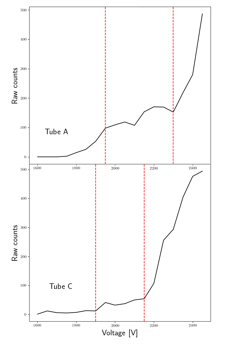
For a Geiger-Müller device, this characterization curve has three main region:
Region I, where the voltage is low enough that only especially high-energy charged particles will create a voltage, which will be proportional to its individual energy;
Region II, where the voltage is high enough to keep the gas close to spontaneously ionizing, and almost every incident charged particle has enough enrgy to create a breakdown;
Region III, where the voltage is so high that it is stripping electrons off of the gas, causing an abundance of false counts that grows with the voltage until all of the gas is ionized.
Region II, also known as the Geiger region, is the most useful one for this experiment, as it gives the most accurate measurement of actual incident muons for a wide range of energies. The three regions are delineated for each of the detectors in Figure 7 based on inspection.
The previous figure indicates that anode voltage of around 2100 V would be ideal for coincidence measurements of muons, because it is a voltage for which both tubes are in their Geiger region. However, due to malfunctions with Tube A and with the backup detector Tube B, we proceeded to use Tube C and an additional detector tube supplied by laboratory supervisor Tyler Morrison.
Given the low detection rates of both of our tubes, we decided used a voltage of 2600 V for all of our coincidence measurements with these two tubes, bringing the detector into Region III. Although this brings our detectors into potentially oversensitive levels, the number of false counts generated is low relative to the improvement in sensitivity, and the probability that two random false counts will occur on each tube independently to create a false coincidence count is minor. The benefit of a higher voltage is a greater sensitivity to lower energy muons, which helps with the second detection of muons after they has been non-trivially damped by thick glass. Although continuous discharge degrades the detectors over time, it is an appropriate measure for the scope of this experiment.
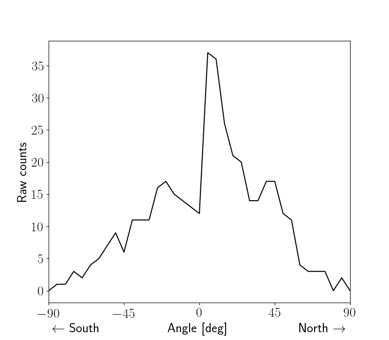
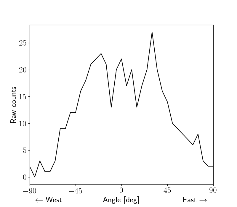
For our measurements of muon incidence, we north-south and east-west angular ranges into \(5^\circ\) steps, and took counts for 12 minutes for each angle. The direct results are plotted in Figures 8 and 9.
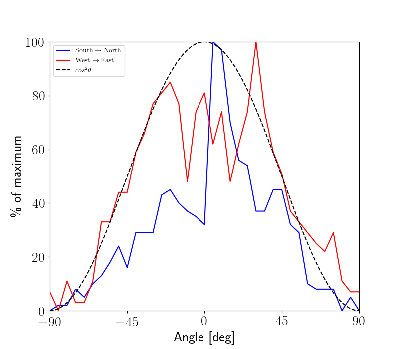
These measurements roughly coincide with the \(cos^2 \theta\) form we expected our distribution to take, as is indicated in Figure 10. This plot scales the "counts" data of both data sets to a percent of maximum – we do not expect that the exact number of particles we detected is representative of the full muon intensity incident on the Earth, so our analysis considers only the dependence on polar angle, with the understanding that a consequent value of the flux has some geometric coefficients in front.
Taking measurements of muons incident in the detector in this experiment is equivalent to sampling a Gaussian distribution of muons. Then, the measurements we take form a Poisson distribution, which has the form
\[P(p,n) = e^{-p} \left( \frac{p^n}{n!} \right),\]
where \(p\) is a random variable (here, the average number of cosmic rays over a time of 12 minutes) and \(n\) can be understood as the average or expected value of the probability. Then, by the properties of the Poisson distribution, each measurement of muon flux has an expectation value and standard deviation of \(\braket{p} = \sigma_p = \sqrt{n}\), where \(n\) is the number of counts in that measurement.
We perform a chi-squared minimization on our east-west and north-south data sets to get best fits of the form \(\cos^bx\) (noting that we have already normalized the amplitude). For this model, we define \(\chi^2\) as the sum:
\[\chi^2 = \sum_{i}^{36} \frac{(\cos^b x_i - y_i)^2}{\sigma_i^2}\]
over all of the data points in the set. Then, \(\chi\) represents some distance between the data and the model that we minimize by our selection of the model \(b\). As stated above, the standard deviation for our purposes here is equal to \(y_i\), the number of counts taken in a sample.
The condition for optimal \(b\) is
\[\frac{\partial \chi^2}{\partial b} = \sum_i^{36} \frac{2 (\cos^b x_i) \ln(\cos x_i) (\cos^b x_i - y_i)}{\sigma_i^2} = 0\]
By approximating \(\cos^b x_i\) as an 8th-order polynomial and solving numerically, we find that \(b=2.55\) for the north-south measurement, and \(b=1.76\) for the east-west measurement. Figures 11 and 12 show this result, each compared with the basic \(b=2\) case.
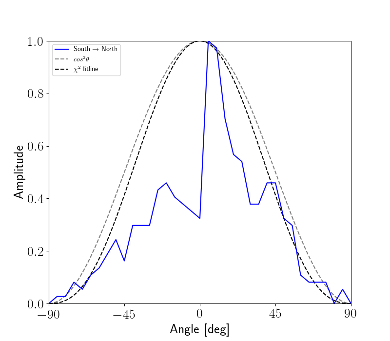
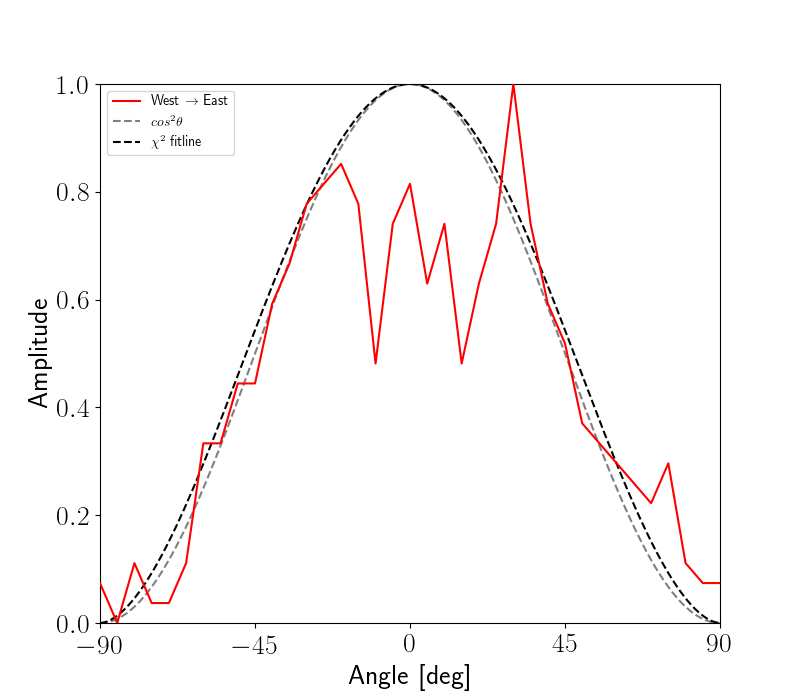
These are very simple, single-term examples of fitting functions. In order to quantify the effect of east-west anisotropy on our measurements, we would need to devise a fitting function that reflects that phenomena, perhaps with an additional odd or antisymmetric term in our model. Therefore we cannot conclusively say whether or not our measurement of muon flux along the east-west axis corroborated our expectations of the effects of the Lorentz force on cosmic ray muons.
Examining the graph of the north-south data in Figure 8, there is a clear distinction in the relative amplitude between the left and right sides of the graph. In fact, the data in this graph was taken starting at the center, moving to the left, and coming back around through the right. Therefore the significant discrepancy between that plot and the theoretical expectation may be the result of some systematic change that built throughout the week or more that was spent taking that data.
In any case, dividing the measurements of an experiment between days or weeks introduces any number of discrepancies that are difficult to predict. The most reliable way to minimize these errors is to increase the number of iterations of the experiment. More data means these random singular events get averaged away in the long run.
There are other limitations and sources of error that exist intrinsically to the experiment. For one, there is no guarantee whatsoever that we are only measuring cosmic ray-derived muons with our detectors. Geiger-Müller tubes are sensitive to any form of ionizing radiation, including any terrestrial sources. The unavoidable dead time and recovery time, combined with the fact that lower-energy muons may not be able to make it into the second tube after getting through the first, mean that the experimental setup will not measure all muons incident on it, which is a source of error.
Finally, our specific issues with questionably build detector tubes and the use of an uncharacterized detector during our data taking mean that there is additional error that is unaccounted for in this analysis.
There are many means not explored here for measuring muons and other cosmic ray products, including Cherenkov counters, scintillators, cloud chambers, emulsion plates, and more. Additionally, there are other observable parameters of these products not considered in this experiment, such as the measuring the energy and counting the particle species.
By focusing on the Geiger-Müller method for radiation detection, which is based in physics familiar to most undergraduate students, we were able to develop our experimental and analytical skills in the course of this project while building on knowledge we have already obtained.
Through the design, fabrication, and execution of our experiment described here, we were able to directly measure the angular dependence of the flux of atmospheric muons, and through statistical analysis, verify our physical expectations for the observations in this experiment.
The author thanks her lab partners and peers, Charles Dickerson, Andrew Essel, and Courtney Watson, for their collaboration in this experiment.
Special thanks to Tyler Morrison and Cristian Cernov for their help, advice, and expertise over the course of this lab.
B. W. Carrol. and D. A. Ostlie, An Introduction to Modern Astrophysics, 2nd ed. (2007) p. 410, 550-553
M. J. Fitzpatrick, Cosmic Ray Detection with a Geiger-Muller Apparatus, (1990)
B. Rossi, Interpretation of Cosmic Ray Phenomena, Rev. Mod. Phys. 20, 537, (1948)
"Nobel Prize in Physics 1936 - Presentation Speech". Nobelprize.org. Nobel Media AB 2014. Web. 30 Apr 2018.
G. Lemaitre and M. S. Vallarta, On Compton’s Latitude Effect of Cosmic Radiation, Phys. Rev. 43, 87, (1933)
P. Sommers and S. Westerhoff, Cosmic ray astronomy, New J. Phys. 11, 055004 (2009)
B. Gutowski, The secret chambers in the Chephren Pyramid (2017)
D. J. Griffiths, Introduction to Electromagnetism 4th ed. (2015)
D. V. S. Murty, TRansducers and Instrumentation, 2nd ed., (2010) p. 424
Janossy, Cosmic Rays (1950) p. 40
P. Horowitz and W. Hill, The Art of Electronics, 2nd ed. (1989) p. 58